Quantum Computing Challenge - Day 7: Quantum Mechanics Fundamentals - Schrödinger Equation, Density Matrices, and Postulates
This post is part of my 21-day quantum computing learning journey, exploring the fundamental laws that govern quantum systems. I dive into the Schrödinger equation, density matrices, and quantum postulates - the mathematical bedrock of quantum computing. Progress: 7/21 days completed. Schrödinger equation: ✓. Density matrices: mastered. Quantum postulates: established.
The Schrödinger Equation: Quantum laws of motion
The Schrödinger equation is quantum mechanics’ equivalent to Newton’s second law, describing how quantum systems evolve over time.
Schrödinger Equation: The Heart of Quantum Evolution
Time-dependent Schrödinger Equation
The time evolution of a quantum state is governed by:
\[iℏ * ∂Ψ(x, t) / ∂t = ˆH * Ψ(x, t)\]Where:
Ψ(x, t)is the wave function at position x and time t.ℏis the reduced Planck constant.ˆHis the Hamiltonian operator.∂Ψ(x, t) / ∂trepresents the time derivative of the wave function.
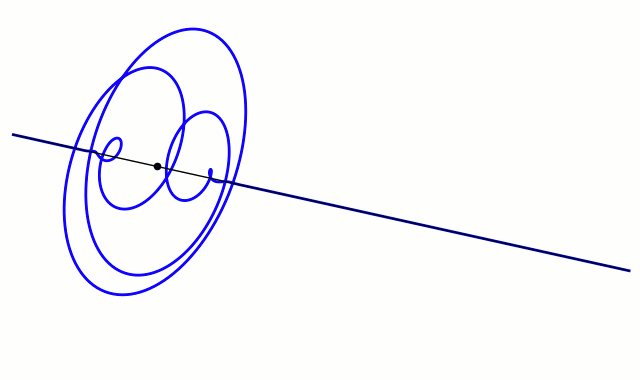
- Complex plot of a wave function that satisfies the nonrelativistic free Schrödinger equation with V = 0. For more details see wave packet
Time-independent Schrödinger Equation
For systems with time-independent potentials, the equation simplifies to:
\[\hat{H} \psi(x) = E \psi(x)\]These solutions — called energy eigenstates — describe stable quantum configurations and are essential in quantum computing, especially for:
- Qubit initialization
- Quantum gates design
- Quantum simulation and chemistry
Each of these three rows is a wave function which satisfies the time-dependent Schrödinger equation for a harmonic oscillator.
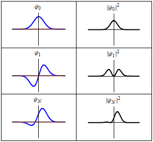
- Quantum harmonic oscillator
imaginary part (red) of the wave function.
Left: The real part (blue) and Right: The probability distribution of finding the particle with this wave function at a given position. The top two rows are examples of stationary states, which correspond to standing waves.
The bottom row is an example of a state which is not a stationary state. The quantum harmonic oscillator is the quantum-mechanical analog of the classical harmonic oscillator.
Because an arbitrary smooth potential can usually be approximated as a harmonic potential at the vicinity of a stable equilibrium point, it is one of the most important model systems in quantum mechanics. Furthermore, it is one of the few quantum-mechanical systems for which an exact, analytical solution is known
Density Matrices: Pure vs Mixed States
Density matrices describe both ideal and realistic quantum systems:
Quantum States: Pure vs. Mixed
| State Type | Expression | Properties |
|---|---|---|
| Pure state | \(\rho = |\psi\rangle\langle\psi|\) | \(\rho^2 = \rho\), maximum coherence |
| Mixed state | \(\rho = \sum_i p_i |\psi_i\rangle\langle\psi_i|\) | \(\rho^2 < \rho\), partial decoherence |
Key Properties:
- Hermitian:
ρ† = ρ - Normalized:
Tr(ρ) = 1 - Positive:
ρ ≥ 0
Mixed states are essential for modeling decoherence and noise in real quantum computers.
The Five Postulates of Quantum Mechanics
| Postulate | Description | Quantum Computing Relevance |
|---|---|---|
| 1. State | System described by \(|\psi\rangle\) in Hilbert space | Qubit superposition states |
| 2. Observable | Physical quantities are Hermitian operators | Measurable quantum properties |
| 3. Measurement | Returns eigenvalues; state collapses | Information extraction |
| 4. Probability | \(P(a_i) = |\langle \psi_i | \psi \rangle|^2\) | Probabilistic outcomes |
| 5. Evolution | Governed by the Schrödinger equation | Unitary quantum gates |
My site is free of ads and trackers. Was this post helpful to you? Why not